Asking a model to be concise is easy. Asking it to be only a little more concise is harder. A useful instruction may remove half the answer when all we wanted was less preamble. Rewriting an adjective can change the result, but it does not give us a dependable scale.
We explored this in ControlPE in 2023: distill a prompt-induced behavior into a LoRA adapter, then adjust its merge weight. The experiments cover concise replies, refusal, and step-by-step reasoning, including settings between a fully applied instruction and no instruction.
Prompt strength control
Prompt optimization usually searches over words. We can rewrite instructions by hand or generate candidates and evaluate them automatically. After finding a useful instruction, however, the most direct choices remain including it or leaving it out. Words such as “slightly” express intent without defining a calibrated amount.
Length makes the problem easy to see. A brevity instruction can shorten replies while also removing explanations. In document question answering, stronger instructions to abstain without evidence can reduce fabrication while increasing refusals on answerable questions. The variable we want to adjust is the behavioral influence of an instruction, rather than its wording alone.
Once an instruction has been chosen, ControlPE learns a parameter update associated with it and exposes a coefficient on that update. The method needs model-weight access and adapter training, so it cannot run through a generation-only API. That effort is more useful when a behavior needs repeated calibration.
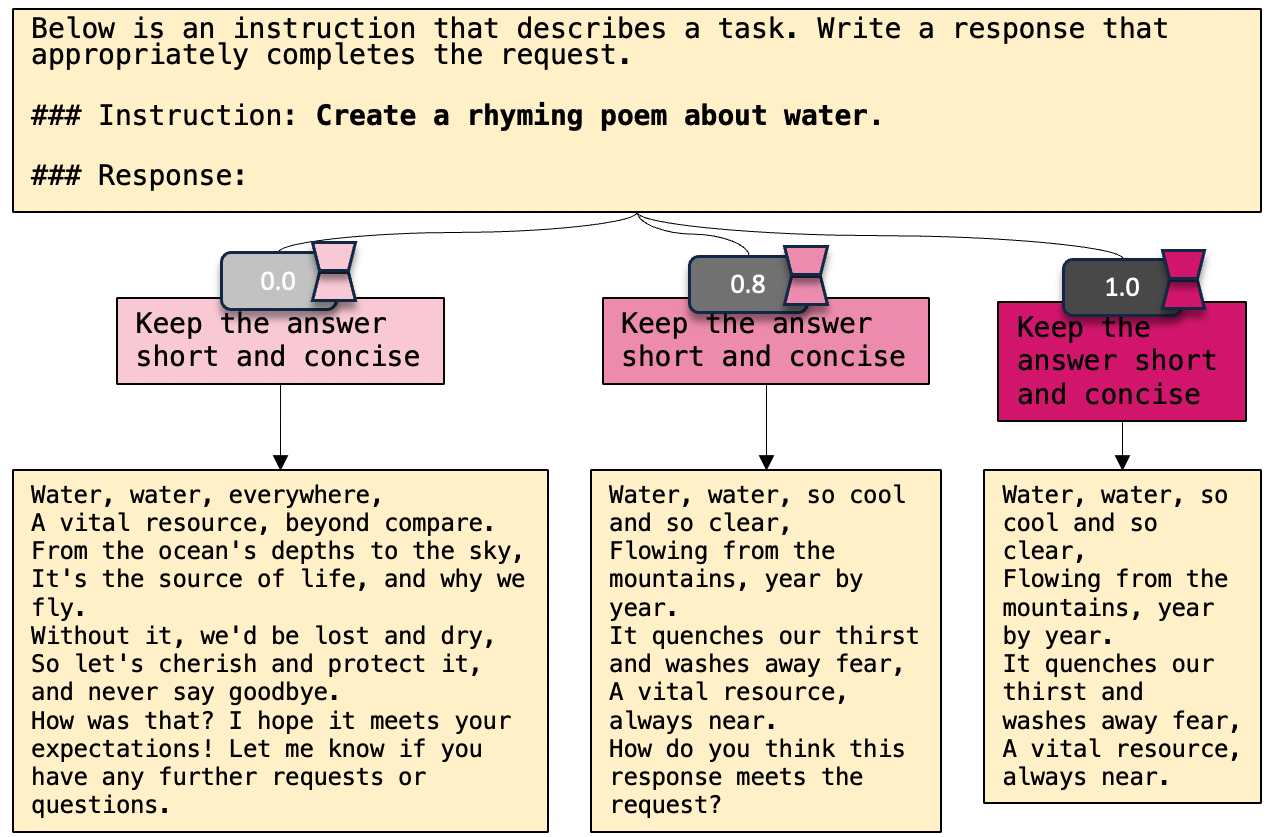
The coefficient is continuous; generated text is not. Changing the coefficient need not change every answer smoothly, or by the same amount. Our curves describe behavior over a set of questions, not an exact word budget for each reply.
Prompt distillation and weight scaling
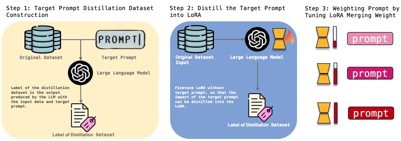
The method has three steps. The important detail is a deliberate difference between the input used to produce labels and the input used to train the adapter.
Generate demonstrations with the target prompt
We start with task inputs, an original prompt template, and a target instruction. The base model sees all three and generates the labels for a distillation dataset. There is no larger external teacher in this procedure: the same model supplies demonstrations under an additional instruction.
The original template organizes the task; the target prompt specifies the behavior to add. For brevity, the labels come from responses generated with a brevity instruction. For step-by-step reasoning, they come from generation with a reasoning instruction. The dataset retains the task input and the generated response.
Distillation still depends on the prompted base model. Poor demonstrations will not supply a missing capability, and shorter labels may omit information. Both task completion and the behavior being transferred need checking.
Train LoRA without the target prompt
We freeze the base model and train LoRA on those input–response pairs. Training uses the original template and task input, but omits the target instruction. The desired response still comes from the prompted generation. The adapter must therefore account for an influence that is no longer present in the text input.
Removing the target instruction during training makes the adapter learn its effect. If the wording stays in the input, the model may continue to rely on it. At inference, the original template and trained adapter should reproduce a similar behavior without repeating the instruction.
Reproduction remains approximate. We fit outputs on finite data; we do not establish that a parameter update and a natural-language instruction are equivalent for every input. The base model, template, and data distribution remain part of the experiment. Changing them calls for another check.
Scale the LoRA weights
LoRA represents a weight update using two low-rank matrices. We attach a coefficient to the resulting update. In the expression below, λ is the coefficient we vary, while s is the adapter’s existing scaling factor. Keeping those concepts separate makes implementation easier to reason about.
At zero, the learned update is absent. At one, it is fully applied. Intermediate values give us a range to scan without retraining. The update is linear in this coefficient; answer length, quality, and refusal behavior need not be.
Scaling both low-rank matrices by λ scales their product by λ squared. The paper compares this with single-matrix scaling and uses the latter in subsequent experiments. Before comparing coefficients between implementations, check which update each coefficient actually applies.
Response length control
The experiments use LLaMA2-7B-chat, with rank-16 LoRA adapters on every attention q_proj and v_proj. Training uses batch size 128, a learning rate of 3e-4, and three epochs. These describe the historical setup, rather than defaults we would automatically recommend for another model.
For length control, the first 10,000 Alpaca instructions supply the distillation inputs. Instructions 10,001–10,100 form the test set. The reported number is the total response-token count for all 100 test instructions, not the mean length of one response.
| Configuration | Total tokens across 100 test responses |
|---|---|
| Original template | 14,766 |
| With the brevity instruction | 7,096 |
| Full distilled LoRA | 6,640 |
The instruction already causes a large change, and the full adapter produces a similar brevity effect. The more useful question is what happens between the endpoints. Scanning the merge weight produces a range of response lengths without choosing another natural-language formulation each time.
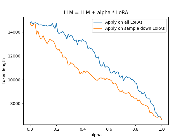
Single-matrix scaling produces an approximately linear aggregate length curve on this test set. Quality was not established at every setting. A deployment evaluation would also need to check essential facts, required reasoning steps, and unusually long replies.
The aggregate hides individual differences. A lookup may already need only one sentence; a multi-step explanation may get shorter by losing a necessary step. The curve can identify a weight range for inspection, but the coefficient is not a fixed length budget for every answer.
Refusals and false refusals
The second experiment uses document question answering. A reply should draw on the supplied material and abstain when that material cannot answer the question. We distill an instruction expressing that requirement, then adjust its influence between answering too readily and refusing too often.
The first 10,000 wikipedia-trivia examples supply distillation inputs. Examples 10,001–10,200 form the test set, with sufficient evidence in 80% of cases and insufficient evidence in 20%. Direct refusal is 0% without the instruction, 27% with it, and 29% with the full distilled adapter.
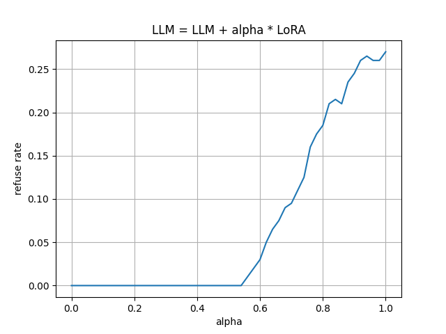
Interpreting 29% against 27% requires knowing which questions were refused. Unsupported questions should be caught without rejecting supported ones. The paper examines refusal precision and recall as well; stronger refusal influence trades them off.
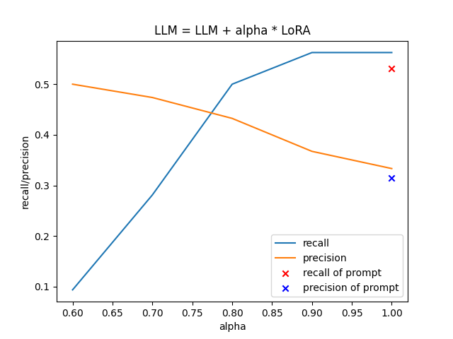
The scoring rule explains another feature of the curve. Direct refusal is counted through a particular explicit response. At weights of 0.1–0.5, some outputs become more cautious or avoid fabrication without using that response. The direct-refusal curve changes more visibly in the 0.6–1.0 range. A low value can therefore describe either continued unsupported answering or a different way of expressing uncertainty.
Refusal needs calibration against evidence availability. Maximizing refusals can favor an unhelpful model; maximizing answers can conceal unsupported claims. Scanning the coefficient makes the trade-off easier to inspect, with answerable and unanswerable cases checked separately.
CoT strength and answer quality
We next distill step-by-step reasoning. The first 10,000 Alpaca instructions again supply the demonstrations, and GSM8K supplies the evaluation task. The distillation data is therefore different from the benchmark; this procedure does not construct labels from GSM8K reference solutions.
| Configuration | GSM8K accuracy |
|---|---|
| Without the step-by-step instruction | 12.6% |
| With the instruction | 14.6% |
| Full distilled LoRA | 14.9% |
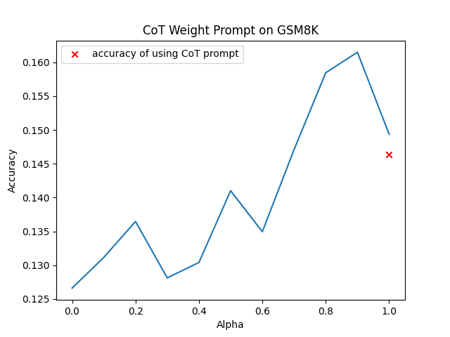
The best region in the weight scan is around 0.8, rather than the fully applied adapter. Even when an instruction helps on average, maximizing its influence need not maximize task accuracy. A stronger tendency to reason changes the generation process without guaranteeing that the final answer improves.
The result near 0.8 belongs to the 7B model and evaluation setup from 2023. Neither that coefficient nor its accuracy gain transfers directly to other reasoning models. The experiment shows why scanning intermediate weights can reveal a useful region missed by a prompted/unprompted comparison.
Combining LoRA adapters
We also combine brevity and refusal control. This experiment reuses the two adapters already trained; it does not train a new adapter for their combination. Written as a sum of updates, the idea is:
The two coefficients scale different updates. They do not make the resulting behaviors independent. Refusals can change response length, and compression can change the wording used to express insufficient evidence. A setting that looks useful along one axis can behave differently once the other adapter is active.
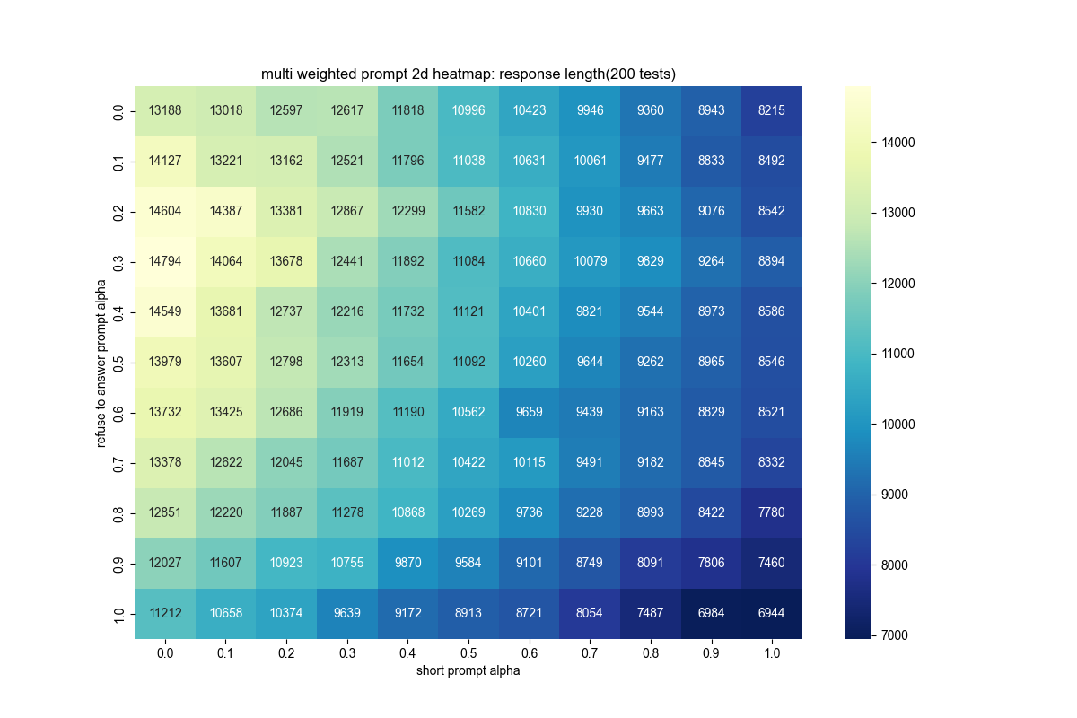
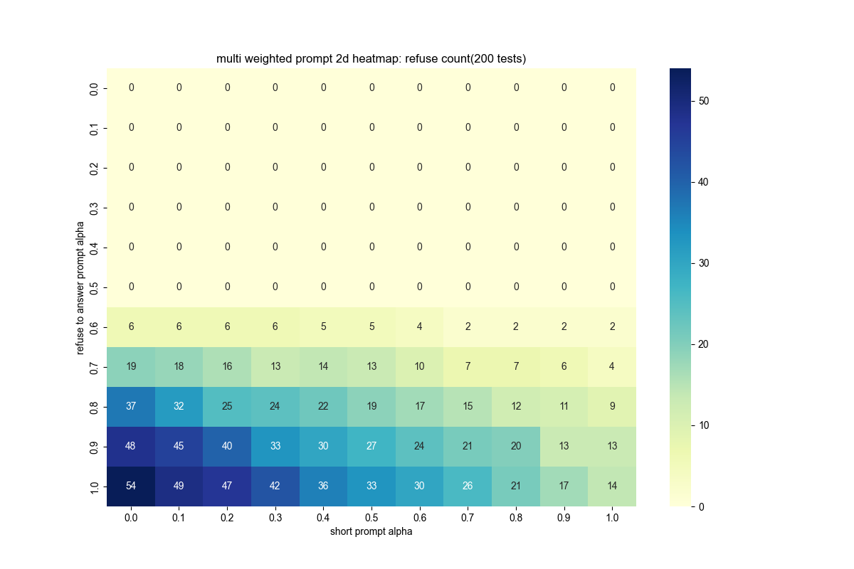
The same 200 DocQA examples are used here. The Alpaca-trained brevity adapter still changes response length on wikipedia-trivia, and refusal remains adjustable. This supports reuse of these two updates, without establishing reliable composition across arbitrary tasks.
A reproduction can compare individual adapter scans with the joint scan. Establish each update’s effect first, then check how it changes in combination. A favorable joint metric may reflect side effects cancelling out rather than improvement in both intended behaviors.
The same reasoning argues against assuming that many adapters will compose cleanly. This experiment covers two specific behaviors, datasets, and updates. Each extra control would introduce another interaction to inspect. The coefficients offer a convenient experimental space, not a guarantee that the space remains easy to calibrate as it grows.
Comparison with other control methods
ControlPE can be confused with soft prompts or prompt tuning. Those also involve continuous parameters, but this method does not replace an input instruction with trainable embeddings. The learned change lives in internal LoRA updates, while the inference input can keep the original text template. Where the update lives matters when deciding whether an existing serving stack can support it.
It also differs from changing sampling temperature. Temperature changes how the output distribution is sampled; ControlPE changes the weights used to compute that distribution. One is a generation setting, the other a learned behavioral update. In a reproduction, I would hold sampling settings fixed while scanning the adapter coefficient so that length changes have an interpretable source.
Check the adapter’s built-in scaling separately from the control coefficient. A tool may fold scaling into a matrix or apply it during the forward pass. Zero should recover the base model and full strength the trained adapter; verify those endpoints before interpreting intermediate values.
Calibration notes
Start calibration with three references: the original template, the target prompt added to it, and the full adapter applied to it. The first pair tests the instruction, and the third tests its transfer. If the full adapter has not learned the behavior, data or training needs attention before a finer weight scan.
Use the same held-out inputs across coefficients. Aggregate metrics help narrow the range; matched questions show which facts or steps each setting removes. For refusal, inspect answerable and unanswerable subsets separately. For reasoning, compare the generated process with final correctness rather than counting reasoning paragraphs.
Selecting a coefficient also calls for a separate final test set. Using one small set both to choose a weight and to report its performance can make calibration look more stable than it is. The paper’s length test has 100 instructions and its refusal test has 200 examples. They reveal useful trends without supporting very fine-grained subgroup conclusions. A domain change needs another check rather than inheriting a historical curve.
For two adapters, begin with a sparse grid, compare it with the individual scans, then refine a useful region. Nearby settings should also preserve task quality and the desired behavior. If only a narrow point works, its sensitivity needs investigation before deployment.
These are suggested calibration checks, not additional product tests reported in the paper. Whether the calibration survives a new base model, template, or question distribution still requires testing.
Use cases and limitations
ControlPE separates instruction choice from strength choice. The prompt defines a behavior, distillation learns a reusable update, and a weight scan finds a suitable range. Each step affects how the final coefficient should be interpreted.
A reproduction should check that the target prompt is used for labels but removed from training inputs, the base model and template remain fixed, scaling affects only the update, and evaluation data is held out. Report task and behavior metrics together to judge whether shorter, more cautious, or longer-reasoning outputs help.
The experiments cover one model family and small tests. They do not guarantee exact control of an individual reply or arbitrary adapter composition. They provide a parameter space to explore when an effective instruction still needs a different strength.